Google Sheets Tutorial
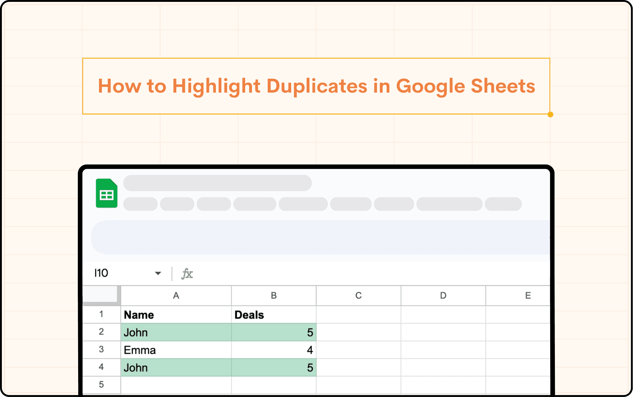
How to Highlight Duplicates in Google Sheets
Learn how to highlight duplicates in Google Sheets. Discover methods for single & multiple columns, plus unique tips with the UNIQUE function.
Table of Contents
Efficiently managing duplicate data is crucial for anyone relying on Google Sheets to monitor performance metrics, manage sales dashboards, or make informed business decisions. Highlighting duplicates in Google Sheets not only streamlines your data management process but also ensures the accuracy and reliability of your data-driven insights. Let’s explore several robust methods to highlight duplicates, providing you with the tools to enhance your data quality significantly.
Prerequisites for highlighting duplicates in Google Sheets
Before you begin to highlight duplicates in Google Sheets, it’s vital to prepare your spreadsheet correctly to ensure accurate results. Here are some preparatory steps:
Remove Existing Formatting: Clear any previous conditional formatting from your cells to avoid conflicts that may arise.
Correct Spacing Issues: Verify that there are no extra spaces before or after your entries, as these can prevent duplicates from being correctly identified.
Exclude Headers from Formulas: When setting up formulas to highlight duplicates, make sure that header rows are not included in the selection.
Selective Highlighting: Sometimes, you may not want to highlight every duplicate. Prioritize which duplicates to mark by adjusting your selections before applying any rules.
Utilize Text Cleaning Functions: Employ the TRIM and CLEAN functions to eliminate unwanted spaces that could obscure duplicate detection.
Top 5 Methods to Highlight Duplicates in Google Sheets
1. Highlight Duplicates in a Single Column
This is one of the simplest ways to start identifying duplicates:
Select the Column: Click on the column that you suspect contains duplicate data, excluding any headers.
Apply Conditional Formatting: Go to Format and click on Conditional formatting, then set up a new rule using the Custom formula is option under Format Rules.
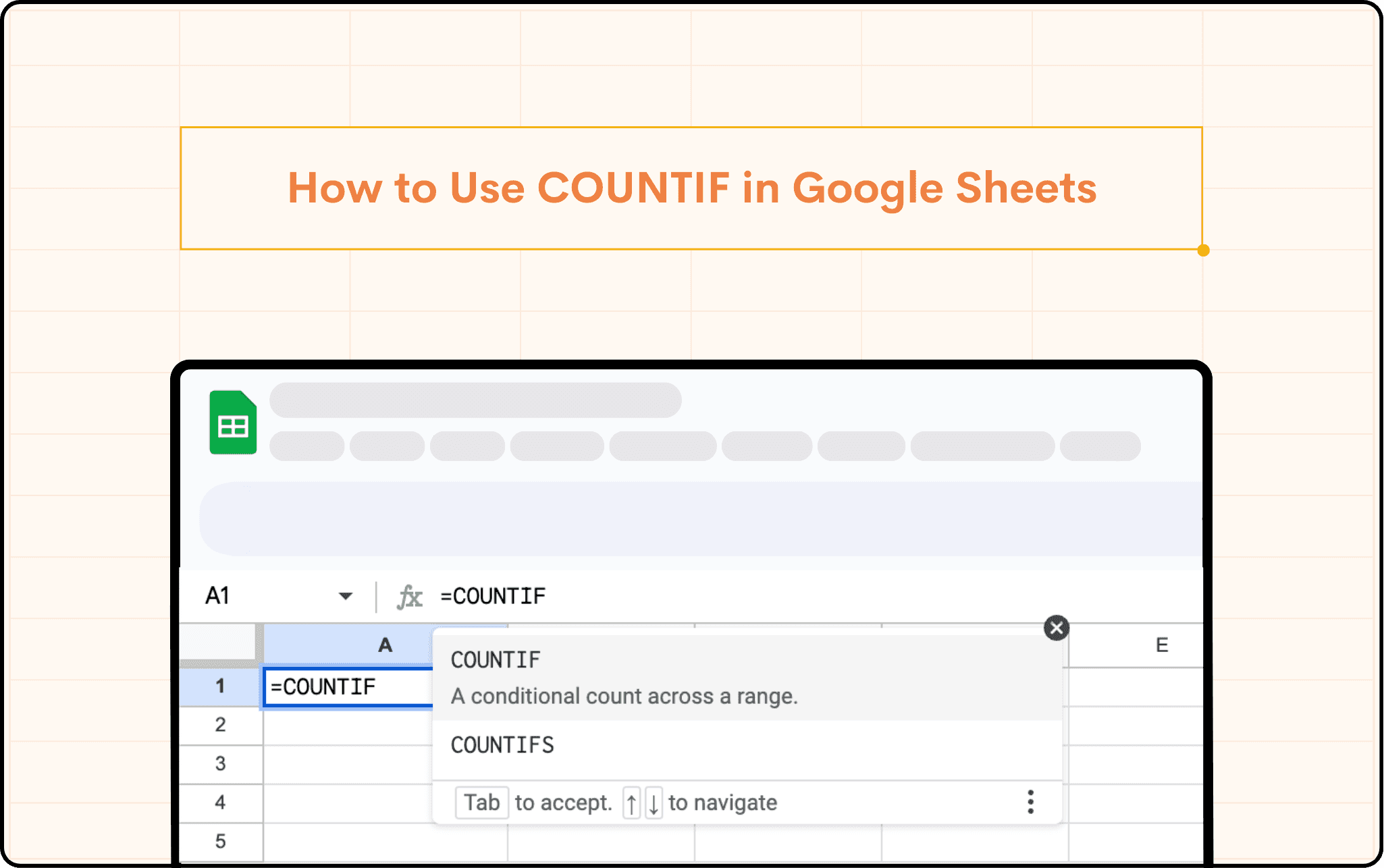
Use the COUNTIF Formula: Input =COUNTIF($A$2:$A, A2)>1 to highlight duplicates. Adjust the range A$2:A according to your data.
Customize the Appearance: Choose how you want the duplicates to be highlighted (color, text style, etc.) and click Done.
This method is dynamic; if duplicates are removed, the formatting will automatically update to reflect the changes.
2. Highlight Duplicates Across Multiple Columns
To extend the duplicate detection across multiple columns, follow these steps:
Define the Range: Select the columns you want to check while avoiding headers.
Apply Conditional Formatting: Same as the single column, Go to Format and click on Conditional formatting, then set up a new rule using the Custom formula is option under Format Rules.
Set Conditional Formatting Rules: Use the formula adjusted for multiple columns =COUNTIF($A$2:$C$100, A2)>1 tailored to the selected range.
Format and Apply: Choose a formatting style for the duplicates, finalize the setup, and click on Done.
3. Identifying Duplicate Rows
Highlighting complete rows of duplicates involves a more comprehensive approach:
Select Appropriate Data Range: Highlight the data range without including the header row.
Apply Conditional Formatting: Navigate to Format and click on Conditional formatting, then set up a new rule using the Custom formula is option under Format Rules.
Combine Data for Unique Identification: Use the formula =COUNTIF(ARRAYFORMULA($A$2:$A&$B$2:$B&$C$2:$C), $A2&$B2&$C2)>1.
Apply Desired Formatting: Select the visual style for highlighting and implement it across the identified duplicates.
This method concatenates the data from multiple columns into a single string per row, making it easier to spot full-row duplicates.
Feeling Confused? Here is a quick explanation of this method:
The formula COUNTIF counts how many times a specific condition is met within a range.
ARRAYFORMULA applies a function to each cell in a range, allowing us to concatenate the values in columns A, B, and C for each row.
$A$2:$A, $B$2:$B, and $C$2:$C represent the ranges in columns A, B, and C where your data is stored.
The & operator concatenates the values in each row of columns A, B, and C into a single string.
$A2&$B2&$C2 concatenates the values in the current row of columns A, B, and C into a single string.
>1 checks if the count of the concatenated strings is greater than 1, indicating that the combination of values has occurred more than once in the data range.
Overall, the formula checks for duplicate combinations of values in columns A, B, and C for each row. If a duplicate combination is found in the current row, it returns TRUE; otherwise, it returns FALSE.
4. Using Additional Criteria for Refined Searches
If your needs require highlighting duplicates based on additional conditions:
In Google Sheets, you have the option to apply additional criteria when highlighting duplicate data. For instance, you can set it up to only identify duplicates for certain values.
To incorporate this, make sure to utilize the star operator (*) within the COUNTIF function. The full syntax will appear as follows:
=(COUNTIF(Range,Criteria)>1) * (Condition 2))
Here is an example:
Implement a formula like =(COUNTIF($A$2:$C$100, $A2)>1)*(COUNTIF($A$2:$C$100, $C2)>1) to use multiple criteria.
This formula checks if both column A and column C in the range from A2 to C100 contain duplicates of the values in the respective rows (row 2 to row 100). If duplicates are found in both columns A and C within the same row, the formula returns TRUE; otherwise, it returns FALSE.
You can refine the formula by adding other conditions or using logical operators to meet specific requirements.
5. Using the UNIQUE Function for Simplicity
The UNIQUE function is particularly useful for smaller data sets:
Just type =UNIQUE(A2:A) in an empty cell within your range to get a list of unique entries.
This approach directly provides you with non-duplicate data, simplifying the process of cleaning up your spreadsheet.
Highlighting duplicates in Google Sheets is a critical step in ensuring the quality of your data. By implementing these easy-to-follow steps, you can enhance the reliability of your operational data, allowing for more accurate analysis and better business decisions.
Say goodbye to tedious data exports! 🚀
Are you tired of spending hours manually exporting CSVs from different tools and importing them into Google Sheets?
StackIt is a data connector for Google Sheets that connects your favorite SaaS tools to Google Sheets automatically. You can get data from these platforms into Google Sheets automatically to build reports that update automatically.
Bid farewell to tedious exports and repetitive tasks. With StackIt, you can add 1 additional day to your week. Try StackIt out for free or schedule a demo.
Efficiently managing duplicate data is crucial for anyone relying on Google Sheets to monitor performance metrics, manage sales dashboards, or make informed business decisions. Highlighting duplicates in Google Sheets not only streamlines your data management process but also ensures the accuracy and reliability of your data-driven insights. Let’s explore several robust methods to highlight duplicates, providing you with the tools to enhance your data quality significantly.
Prerequisites for highlighting duplicates in Google Sheets
Before you begin to highlight duplicates in Google Sheets, it’s vital to prepare your spreadsheet correctly to ensure accurate results. Here are some preparatory steps:
Remove Existing Formatting: Clear any previous conditional formatting from your cells to avoid conflicts that may arise.
Correct Spacing Issues: Verify that there are no extra spaces before or after your entries, as these can prevent duplicates from being correctly identified.
Exclude Headers from Formulas: When setting up formulas to highlight duplicates, make sure that header rows are not included in the selection.
Selective Highlighting: Sometimes, you may not want to highlight every duplicate. Prioritize which duplicates to mark by adjusting your selections before applying any rules.
Utilize Text Cleaning Functions: Employ the TRIM and CLEAN functions to eliminate unwanted spaces that could obscure duplicate detection.
Top 5 Methods to Highlight Duplicates in Google Sheets
1. Highlight Duplicates in a Single Column
This is one of the simplest ways to start identifying duplicates:
Select the Column: Click on the column that you suspect contains duplicate data, excluding any headers.
Apply Conditional Formatting: Go to Format and click on Conditional formatting, then set up a new rule using the Custom formula is option under Format Rules.
Use the COUNTIF Formula: Input =COUNTIF($A$2:$A, A2)>1 to highlight duplicates. Adjust the range A$2:A according to your data.
Customize the Appearance: Choose how you want the duplicates to be highlighted (color, text style, etc.) and click Done.
This method is dynamic; if duplicates are removed, the formatting will automatically update to reflect the changes.
2. Highlight Duplicates Across Multiple Columns
To extend the duplicate detection across multiple columns, follow these steps:
Define the Range: Select the columns you want to check while avoiding headers.
Apply Conditional Formatting: Same as the single column, Go to Format and click on Conditional formatting, then set up a new rule using the Custom formula is option under Format Rules.
Set Conditional Formatting Rules: Use the formula adjusted for multiple columns =COUNTIF($A$2:$C$100, A2)>1 tailored to the selected range.
Format and Apply: Choose a formatting style for the duplicates, finalize the setup, and click on Done.
3. Identifying Duplicate Rows
Highlighting complete rows of duplicates involves a more comprehensive approach:
Select Appropriate Data Range: Highlight the data range without including the header row.
Apply Conditional Formatting: Navigate to Format and click on Conditional formatting, then set up a new rule using the Custom formula is option under Format Rules.
Combine Data for Unique Identification: Use the formula =COUNTIF(ARRAYFORMULA($A$2:$A&$B$2:$B&$C$2:$C), $A2&$B2&$C2)>1.
Apply Desired Formatting: Select the visual style for highlighting and implement it across the identified duplicates.
This method concatenates the data from multiple columns into a single string per row, making it easier to spot full-row duplicates.
Feeling Confused? Here is a quick explanation of this method:
The formula COUNTIF counts how many times a specific condition is met within a range.
ARRAYFORMULA applies a function to each cell in a range, allowing us to concatenate the values in columns A, B, and C for each row.
$A$2:$A, $B$2:$B, and $C$2:$C represent the ranges in columns A, B, and C where your data is stored.
The & operator concatenates the values in each row of columns A, B, and C into a single string.
$A2&$B2&$C2 concatenates the values in the current row of columns A, B, and C into a single string.
>1 checks if the count of the concatenated strings is greater than 1, indicating that the combination of values has occurred more than once in the data range.
Overall, the formula checks for duplicate combinations of values in columns A, B, and C for each row. If a duplicate combination is found in the current row, it returns TRUE; otherwise, it returns FALSE.
4. Using Additional Criteria for Refined Searches
If your needs require highlighting duplicates based on additional conditions:
In Google Sheets, you have the option to apply additional criteria when highlighting duplicate data. For instance, you can set it up to only identify duplicates for certain values.
To incorporate this, make sure to utilize the star operator (*) within the COUNTIF function. The full syntax will appear as follows:
=(COUNTIF(Range,Criteria)>1) * (Condition 2))
Here is an example:
Implement a formula like =(COUNTIF($A$2:$C$100, $A2)>1)*(COUNTIF($A$2:$C$100, $C2)>1) to use multiple criteria.
This formula checks if both column A and column C in the range from A2 to C100 contain duplicates of the values in the respective rows (row 2 to row 100). If duplicates are found in both columns A and C within the same row, the formula returns TRUE; otherwise, it returns FALSE.
You can refine the formula by adding other conditions or using logical operators to meet specific requirements.
5. Using the UNIQUE Function for Simplicity
The UNIQUE function is particularly useful for smaller data sets:
Just type =UNIQUE(A2:A) in an empty cell within your range to get a list of unique entries.
This approach directly provides you with non-duplicate data, simplifying the process of cleaning up your spreadsheet.
Highlighting duplicates in Google Sheets is a critical step in ensuring the quality of your data. By implementing these easy-to-follow steps, you can enhance the reliability of your operational data, allowing for more accurate analysis and better business decisions.
Say goodbye to tedious data exports! 🚀
Are you tired of spending hours manually exporting CSVs from different tools and importing them into Google Sheets?
StackIt is a data connector for Google Sheets that connects your favorite SaaS tools to Google Sheets automatically. You can get data from these platforms into Google Sheets automatically to build reports that update automatically.
Bid farewell to tedious exports and repetitive tasks. With StackIt, you can add 1 additional day to your week. Try StackIt out for free or schedule a demo.
FAQs
Can I highlight only the second or subsequent instances of duplicates, leaving the first instance unhighlighted?
Can I highlight only the second or subsequent instances of duplicates, leaving the first instance unhighlighted?
How can I remove duplicates after highlighting them?
How can I remove duplicates after highlighting them?
Can I highlight duplicates across multiple sheets?
Can I highlight duplicates across multiple sheets?
Automatic Data Pulls
Visual Data Preview
Set Alerts
other related blogs
Try it now